Power and Responsibility: 圣彼得堡悖论

圣彼得堡悖论概述

　　圣彼得堡悖论是决策论中的一个悖论。
　　圣彼得堡悖论是数学家丹尼尔·伯努利（Daniel Bernoulli）的表兄尼古拉·伯努利（Daniel Bernoulli）在１７３８提出的一个概率期望值悖论，它来自于一种掷币游戏，即圣彼得堡游戏。设定掷出正面或者反面为成功，游戏者如果第一次投掷成功，得奖金２元，游戏结束；第一次若不成功，继续投掷，第二次成功得奖金４元，游戏结束；这样，游戏者如果投掷不成功就反复继续投掷，直到成功，游戏结束。如果第ｎ次投掷成功，得奖金２的ｎ次方元，游戏结束。按照概率期望值的计算方法，将每一个可能结果的得奖值乘以该结果发生的概率即可得到该结果奖值的期望值。游戏的期望值即为所有可能结果的期望值之和。随着ｎ的增大，以后的结果虽然概率很小，但是其奖值越来越大，每一个结果的期望值均为1，所有可能结果的得奖期望值之和，即游戏的期望值，将为“无穷大”。按照概率的理论，多次试验的结果将会接近于其数学期望。但是实际的投掷结果和计算都表明，多次投掷的结果，其平均值最多也就是几十元。正如Hacking（１９８０）所说：“没有人愿意花２５元去参加一次这样的游戏。”这就出现了计算的期望值与实际情况的“矛盾”，问题在哪里? 实际在游戏过程中，游戏的收费应该是多少？决策理论的期望值准则在这里还成立吗？这是不是给“期望值准则”提出了严峻的挑战？正确认识和解决这一矛盾对于人们认识随机现象、发展决策理论和指导实际决策无疑具有重大意义。
　　圣彼得堡问题对于决策工作者的启示在于，许多悖论问题可以归为数学问题，但它同时又是一个思维科学和哲学问题。悖论问题的实质是人类自身思维的矛盾性。从广义上讲，悖论不仅包括人们思维成果之间的矛盾，也包括思维成果与现实世界的明显的矛盾性。对于各个学科各个层次的悖论的研究，历来是科学理论发展的动力。圣彼得堡悖论所反映的人类自身思维的矛盾性，首先具有一定的哲学研究的意义；其次它反映了决策理论和实际之间的根本差别。人们总是不自觉地把模型与实际问题进行比较，但决策理论模型与实际问题并不是一个东西；圣彼得堡问题的理论模型是一个概率模型，它不仅是一种理论模型，而且本身就是一种统计的 “近似的”模型。在实际问题涉及到无穷大的时候，连这种近似也变得不可能了。

实验的论文解释

　　丹尼尔·伯努利对这个悖论的解答在１７３８年的论文里，提出了效用的概念以挑战以金额期望值为决策标准，论文主要包括两条原理：
　　１、边际效用递减原理：一个人对于财富的占有多多益善，即效用函数一阶导数大于零；随着财富的增加，满足程度的增加速度不断下降，效用函数二阶导数小于零。
　　２、最大效用原理：在风险和不确定条件下，个人的决策行为准则是为了获得最大期望效用值而非最大期望金额值。

圣彼得堡悖论的消解历史

　　圣彼得堡悖论的提出已有２００多年了，所提出的消解方法大致可以归纳为以下几种观点：
　　（一）边际效用递减论
　　Daniel Bernoulli在提出这个问题的时候就给出一种解决办法。他认为游戏的期望值计算不应该是金钱，而应该是金钱的期望效用，即利用众所周知的“期望效用递减律”，将金钱的效用测度函数用货币值的对数来表示：效用=log（货币值）。所有结果的效用期望值之和将为一个有限值log(4)≈ 0.60206，如果这里的效用函数符合实际，则理性决策应以4元为界。这一解释其实并不能令人满意。姑且假定“效用递减律”是对的，金钱的效用可以用货币值的对数来表示。但是如果把奖金额变动一下，将奖金额提高为l0的2n次方(n=3时，奖金为108)，则其效用的期望值仍为无穷大，新的悖论又出现了当然，我们并不清楚效用值与货币值之间究竟有什么样的关系，不过只要我们按照效用的2n倍增加奖金，悖论就总是存在。
　　（二）风险厌恶论
　　圣彼得堡悖论对于奖金额大小没有限制，比如连续投掷４０次才成功的话，奖金为1.1万亿元。但是这一奖金出现的概率极小，1.1万亿次才可能出现一次。实际上，游戏有一半的机会，其奖金为２元，四分之三的机会得奖4元和2元。奖金越少，机会越大，奖金越大，机会越小。如果以前面 Hacking所说。花25元的费用冒险参与游戏将是非常愚蠢的，虽有得大奖的机会，但是风险太大。因此，考虑采用风险厌恶因素的方法可以消解矛盾。 Pual Weirich就提出在期望值计算中加入一种风险厌恶因子，并得出了游戏费用的有限期望值，认为这种方法实际上解决了该悖论。
　　但是这种方法也并不十分完美。首先，并非所有人都是风险厌恶的，相反有很多人喜欢冒险。如每期必买的彩票，以及Casino（卡西诺）纸牌游戏，其价格都高于得奖的期望值。你也可以说这些喜欢冒险买彩票和赌博的人是非理性的，可他们自有乐趣，喜欢这样的风险刺激。总之，风险厌恶的观点很难解释清楚实际游戏平均值非常有限的问题。退一步说，即便承认风险厌恶的观点，矛盾仍然不能消除。我们仍然可以调整奖金额，最后，考虑风险厌恶情况的期望值仍然是无穷大而与实际情况不符。
　　　（三）效用上限论
　　对前两种观点的反驳，我们采用了增加奖金额的方法来补偿效用的递减和风险厌恶，两者均是假定效用可以无限增加。也有一种观点认为奖金的效用可能有一个上限，这样，期望效用之和就有了一个极限值。Menger认为效用上限是惟一能消解该悖论的方法。设效用值等于货币值，上限为１００单位，则游戏的期望效用为7.56l25，如表3所示。也许这里的效用上限太小了，不过我们可以任意选定一个更大的值比如225 。有多人如Russell Har—din (1982)，W illiam G uNtaNon (1994)，Richard Jeffrey(1983)等都赞成这样的观点。不过这种效用上限的观点似乎不太令人信服。效用上限与效用递减不同，或许你认为有２２５的钱够自己花的了，可是钱并不能给我们带来所有的效用，有些东西不是钱所能买来的。效用上限意味着再也没有价值可以添加了。但是一个人有了钱，还希望他的朋友、亲戚也像他一样富有；同一个城市里的人和他一样富有。而效用上限论认为到了这一上限他们就不用再做任何交易了，看起来这并不能成立。对有些人来讲，似乎期望和需求并不是无限增加的，对于现有的有限需求他们已经满足了。他们觉得这里的游戏期望效用值确实是有限的。不过是不是确实有这样的人还是一个不确定的问题，或者是个经验性的问题。但认为“越多越好”的人确实是存在的。对于决策准则这样的理性选择的理论，不能基于可疑的和经验性的判断而加以限制，因而期望有限论不足以消解这里的矛盾。
　　　（四）结果有限论
　　Gustason认为，要避免矛盾，必须对期望值概念进行限制，其一是限制其结果的数目；其二是把其结果值的大小限制在一定的范围内。这是典型的结果有限论，这一观点是从实际出发的。因为实际上，游戏的投掷次数总是有限的数。比如对游戏设定某一个投掷的上限数Ｌ，在投掷到这个数的时候，如果仍然没有成功，也结束游戏，不管你还能再投多少，就按照Ｌ付钱。因为你即便不设定Ｌ，实际上也总有投到头的时候，人的寿命总是有限的，任何原因都可以使得游戏中止。现在设定了上限，期望值自然也就可以计算了。
　　问题是，这已经不是原来的那种游戏了！同时也并没有证明原来的游戏期望值不是无限大。原来的游戏到底存在吗？ Jeffrey说：“任何提供这一游戏的人都是一个骗子，谁也没有无限大的银行！”是说实际上没有这种游戏吗？恐怕这也不见的。如果我邀请你玩这种游戏，你说我实际上不是在这样做吗? 或者说我实际上邀请你玩的不是这种游戏而是另外的什么游戏? 很多游戏场提供许多概率极小、奖金额极大几乎不可能的游戏，他们仍然在经营、在赚钱，照样吃饭睡觉，一点儿也不担心哪一天会欠下一屁股债，崩盘倒闭。
　　Jeffrey在这样说的时候，实际上是承认了圣彼得堡游戏的期望值是无穷大了。认为游戏厅不提供这样的游戏，正是因为他们认为其期望值是无穷大，迟早他们会因此而破产倒闭。这正是用了常规的决策理论，而反过来又说这种游戏实际上不存在，应该排除在期望值概念之外。因此，用限制期望值概念的方法并不能消解悖论。
　　不能限制期望值概念的原因还有很多。比如，我们不能用限制期望值概念的方法仅把圣彼得堡游戏排除在外，而应该是通用的。在人寿保险中，有一个险种根据保险人的年龄，每长一岁给付一定的赔付金额。采用人类寿命的经验曲线给出每个年龄的生存机会。大于１４０岁的生存率已经没有经验可以借鉴，但可以采用一定的函数将生存年龄扩展至无穷大，当然其生存率趋向于零。注意到这里的给付金额也是无限的，但是其在期望值计算方面并没有出现什么问题。

问题的本质与悖论的消解

　　所谓悖论，《辞海》中的定义是：“一命题Ｂ，如果承认Ｂ，可推得非Ｂ，反之，如果承认非Ｂ，又可推得Ｂ，称命题Ｂ为一悖论。”可见，作为一种推理的矛盾现象，悖论是人们自己制造出来的。现在已经有人证明，这种意义上的悖论是不存在的。一个命题是一个具有真假的判断语句，如果一个命题Ｂ和非Ｂ能够相互推出，则Ｂ要么是非真非假的单义句，要么是非真非假的多义句。所以，悖论作为人类思维系统的一种矛盾形式，它的消解必须从人们思维系统自身的矛盾性和不完善性着手，需要人类战胜和超越自己。历史上一次一次的悖论的消解，提出了更完备的公理系统，完善了人类的思维和科学系统，使得科学得到进一步的发展。圣彼得堡悖论也是一样。
　　　（一）对圣彼得堡悖论各种消解观点的评述
　　综合上述悖论的消解观点，效用递减论符合了“边际效用递减律”，能够在一定程度上解决实际问题，但是却绕开了问题的基本面。圣彼得堡游戏的期望值到底是多少并没有真正得到解决；风险厌恶论，犯了同样的错误，只不过是用风险因子替换了效用函数，实际上只是一种风险效用；效用上限论和结果上限论试图回避问题的无限性，篡改了原问题，自然也不可能解决问题。这些观点都是从实际出发的，但都没有触及人们的思维系统，不能冲破自己思想的牢笼，即便解决了这一悖论，又会有新的悖论出现。
　　　（二）最后的消解
　　从上述圣彼得堡悖论的消解方法来看，其效果都不是十分理想，都没有真正解决问题。但是正是这些努力，是我们认识到仅从实际出发是不能解决问题的，而最合理的解释就是— — 保留期望值的定义，调整我们的思维。当我们这样做的时候，圣彼得堡悖论就不再是一个悖论了！理论上期望值的计算没有什么错误，我们需要承认它的期望值是无穷大；而实际上它的均值又不可能是无穷大，因为它是样本均值，样本均值随着样本容量的增加，以概率收敛于其期望值。这都是正常的，它们本身就是应该有差距的！至于差距应该有多大，在小于无穷大的时候，样本均值随着实验次数的增多，越来越接近总体均值（或理论均值），圣彼得堡游戏不正是这样的吗？而在总体均值是无穷大的时候，我们如何让样本均值如何接近无穷大呢？非得是我们认为的很大很大吗？再大也不是无穷大，和现在也没有区别，我们平时的“大小”概念已经不适应了。涉及无穷大概念比较的时候，就需要用相应的比较方法。圣彼得堡游戏的结果集合是一个无穷集合，而实际实验的样本是一个有穷集合，它们是不能用现有的办法比较的。
　　利用电脑进行模拟试验的结果说明，实际试验的平均值— — 样本均值是随着实验次数的增加而变化的。在大量实验以后，其实验均值X可以近似表示为X≈logn/log2，可见当实验次数趋向无穷大的时候，样本均值也趋向无穷大。比如100万即106次实验的平均值约等于6/0.301=19.9，即 20元左右；要样本均值达到1 000元，实验次数就要达到10332，这时候有可能出现的最高投掷次数约为1000次左右，相应的最高赔付金额为，已经达到了天文数字了。如果随着实验次数趋向无穷大，趋向于无穷大的速度是慢多了。

对决策理论与现实的启示

　　虽然圣彼得堡游戏问题只是一个具体问题，但是类似的实际决策问题是存在的。它们起码是可观察的，其观察值确实也是存在的。而且它确实也给决策的期望值准则提出了挑战，所提出的问题需要我们给予解答。通过上述问题的消解，我们至少可以给出下列有关问题的答案和启示。
　　首先，理论上应该承认圣彼得堡游戏的“数学期望”是无穷大的。但理论与实际是有差别的，在涉及无穷大决策问题的时候，必须注意这种差别。
　　其次，实际试验中随着游戏试验次数的增加，其均值将会越来越大，并与实验次数呈对数关系，即样本均值=log2(实验次数)=log(实验次数)/log2。
　　再次，实际问题的解决还是要根据具体问题进行具体分析。前面的圣彼得堡悖论消解方法都是很实用的方法。也--I以设计其他方法，比如可以运用“实际推断原理”，根据实验次数n设定一个相应的“小概率”，对于圣彼得堡问题来讲，是一个很实际的方法；或者建立一个近似模型，比如确定一个最大可能成功的投掷次数n，将投掷n+1次以后的概率设为1 / 2k，仍然符合概率分布的条件（所有结果的概率之和等于１）等等。
　　最后，圣彼得堡问题对于决策工作者的启示在于，许多悖论问题可以归为数学问题，但它同时又是一个思维科学和哲学问题。悖论问题的实质是人类自身思维的矛盾性。从广义上讲，悖论不仅包括人们思维成果之间的矛盾，也包括思维成果与现实世界的明显的矛盾性。对于各个学科各个层次的悖论的研究，历来是科学理论发展的动力。圣彼得堡悖论所反映的人类自身思维的矛盾性，首先具有一定的哲学研究的意义；其次它反映了决策理论和实际之间的根本差别。人们总是不自觉地把模型与实际问题进行比较，但决策理论模型与实际问题并不是一个东西；圣彼得堡问题的理论模型是一个概率模型，它不仅是一种理论模型，而且本身就是一种统计的 “近似的”模型。在实际问题涉及到无穷大的时候，连这种近似也变得不可能了。
　　决策科学是一门应用学科，它的研究需要自然科学和社会科学的各种基础理论和方法，包括数学方法。这些方法都具有很强的理论性和高度抽象性。但是，决策科学更是一门应用性、实践性很强的学科，要求决策理论与决策实践紧密结合。因此，我们在决策理论的研究和解决实际问题的时候，应高度重视理论和实践的关系。理论模型的建立，既要源于实践，又不能囿于实践，发挥主观创造力，才能有所突破，有所建立.

Solutions of the paradox

There are different approaches for solving the paradox.

Expected utility theory

The classical resolution of the paradox involved the explicit introduction of a utility function, an expected utility hypothesis, and the presumption of diminishing marginal utility of money.

In Daniel Bernoulli's own words:

The determination of the value of an item must not be based on the price, but rather on the utility it yields…. There is no doubt that a gain of one thousand ducats is more significant to the pauper than to a rich man though both gain the same amount.

A common utility model, suggested by Bernoulli himself, is the logarithmic function u(w) = ln(w) (known as “log utility”). It is a function of the gambler’s total wealth w, and the concept of diminishing marginal utility of money is built into it. By the expected utility hypothesis, expected utilities can be calculated the same way expected values are. For each possible event, the change in utility ln(wealth after the event) - ln(wealth before the event) will be weighted by the probability of that event occurring. Let c be the cost charged to enter the game. The expected utility of the lottery now converges to a finite value:

$EU=\sum_{k=1}^\infty \frac{\ln(w+2^{k-1}-c) - \ln(w)}{2^k} < \infty \,.$

This formula gives an implicit relationship between the gambler's wealth and how much he should be willing to pay to play (specifically, any c that gives a positive expected utility). For example, with log utility a millionaire should be willing to pay up to $10.94, a person with $1000 should pay up to $5.94, a person with $2 should pay up to $2, and a person with $0.60 should borrow $0.87 and pay up to $1.47.

Before Daniel Bernoulli published, in 1728, another Swiss mathematician, Gabriel Cramer, had already found parts of this idea (also motivated by the St. Petersburg Paradox) in stating that

the mathematicians estimate money in proportion to its quantity, and men of good sense in proportion to the usage that they may make of it.

He demonstrated in a letter to Nicolas Bernoulli[1] that a square root function describing the diminishing marginal benefit of gains can resolve the problem. However, unlike Daniel Bernoulli, he did not consider the total wealth of a person, but only the gain by the lottery.

This solution by Cramer and Bernoulli, however, is not yet completely satisfying, since the lottery can easily be changed in a way such that the paradox reappears: To this aim, we just need to change the game so that it gives the (even larger) payoff $e^{2^k}$ . Again, the game should be worth an infinite amount. More generally, one can find a lottery that allows for a variant of the St. Petersburg paradox for every unbounded utility function, as was first pointed out by (Menger, 1934).

There are basically two ways of solving this generalized paradox, which is sometimes called the Super St. Petersburg paradox:

We can take into account that a casino would only offer lotteries with a finite expected value. Under this restriction, it has been proved that the St. Petersburg paradox disappears as long as the utility function is concave, which translates into the assumption that people are (at least for high stakes) risk averse [Compare (Arrow, 1974)].

We can assume that the utility function has an upper bound. Cramer had, in fact, also suggested a simple bounding under which all sums of money beyond some point would have equal utility (id est that the marginal utility of money would go to zero),(Bernoulli 1738) but a utility function need not become constant beyond some point to be bounded; for example the function $u (x) = x / (x + 1)$ is bounded above by 1, yet strictly increasing.

Recently, expected utility theory has been extended to arrive at more behavioral decision models. In some of these new theories, as in Cumulative Prospect Theory, the St. Petersburg paradox again appears in certain cases, even when the utility function is concave, but not if it is bounded (Rieger and Wang, 2006).

Probability weighting

Nicolas Bernoulli himself proposed an alternative idea for solving the paradox. He conjectured that people will neglect unlikely events[2]. Since in the St. Petersburg lottery only unlikely events yield the high prizes that lead to an infinite expected value, this could resolve the paradox. The idea of probability weighting resurfaced much later in the work on prospect theory by Daniel Kahneman and Amos Tversky. However, their experiments indicated that, very much to the contrary, people tend to overweight small probability events. Therefore the proposed solution by Nicolas Bernoulli is nowadays not considered to be satisfactory.

Rejection of mathematical expectation

Various authors, including Jean le Rond d'Alembert and John Maynard Keynes, have rejected maximization of expectation (even of utility) as a proper rule of conduct. Keynes, in particular, insisted that the relative risk of an alternative could be sufficiently high to reject it even were its expectation enormous.

One can't buy what isn't sold

Some economists resolve the paradox by arguing that, even if an entity had infinite resources, the game would never be offered. If the lottery represents an infinite expected gain to the player, then it also represents an infinite expected loss to the host. No one could be observed paying to play the game because it would never be offered. As Paul Samuelson describes the argument:

Paul will never be willing to give as much as Peter will demand for such a contract; and hence the indicated activity will take place at the equilibrium level of zero intensity. (Samuelson, 1960)

(// Good Explanation)

Finite St. Petersburg lotteries

The classical St. Petersburg lottery assumes that the casino has infinite resources. This assumption is often criticized as unrealistic, particularly in connection with the paradox, which involves the reactions of ordinary people to the lottery. Of course, the resources of an actual casino (or any other potential backer of the lottery) are finite. More importantly, the expected value of the lottery only grows logarithmically with the resources of the casino. As a result, the expected value of the lottery, even when played against a casino with the largest resources realistically conceivable, is quite modest. If the total resources (or total maximum jackpot) of the casino are W dollars, then L = 1 + floor(log₂(W)) is the maximum number of times the casino can play before it no longer covers the next bet. The expected value E of the lottery then becomes:

$\begin{align} E &= \sum_{k=0}^\infty \frac{1}{2^{k+1}}\cdot \min(2^k, W) \\ &= \sum_{k=0}^{L-1} \frac{1}{2^{k+1}}\cdot 2^k ~+~ \sum_{k=L}^\infty \frac{1}{2^{k+1}}\cdot W \\ &= \frac{L}{2} ~+~ \frac{W}{2^L}\,\,. \end{align}$

The following table shows the expected value E of the game with various potential backers and their bankroll W (with the assumption that if you win more than the bankroll you will be paid what the bank has):

Backer	Bankroll	Expected value of lottery
Friendly game	$100	$4.28
Millionaire	$1,000,000	$10.95
Billionaire	$1,000,000,000	$15.93
Bill Gates (2008)	$58,000,000,000	$18.84
U.S. GDP (2007)	$13.8 trillion	$22.79
World GDP (2007)	$54.3 trillion	$23.77
Googolaire	$10¹⁰⁰	$166.50

Notes: The estimated net worth of Bill Gates is from Forbes. The GDP data are as estimated for 2007 by the International Monetary Fund, where one trillion dollars equals $10¹² (one million times one million dollars). A “googolaire” is a hypothetical person worth a googol dollars ($10¹⁰⁰).

A rational person might not find the lottery worth even the modest amounts in the above table, suggesting that the naive decision model of the expected return causes essentially the same problems as for the infinite lottery. Even so, the possible discrepancy between theory and reality is far less dramatic.

The assumption of infinite resources can produce other apparent paradoxes in economics. See martingale (roulette system) and gambler's ruin.

[edit] Iterated St. Petersburg lottery

A typical graph of average winnings over one course of a St. Petersburg Paradox lottery shows how occasional large payoffs lead to an overall very slow rise in average winnings. After 20,000 gameplays in this simulation the average winning per lottery was just under 8 dollars. The graph encapsulates the paradox of the lottery: The overall upward slope in the average winnings graph shows that average winnings tend upward to infinity, but the slowness of the rise in average winnings (a rise that becomes yet slower as gameplay progresses) indicates that a tremendously huge number of lottery plays will be required to reach average winnings of even modest size.

Players may assign a higher value to the game when the lottery is repeatedly played. This can be seen by simulating a typical series of lotteries and accumulating the returns; compare the illustration (right).

If the expected payout from playing the game once is E₁, the expected average per-game payout from playing the game n times is:

$E_n = E_1 + \tfrac{1}{2} \left(\log_2 n \right)\,.$

Since E₁ is infinite, E_n is infinite as well. Nevertheless, expressing E_n in this way shows that n, the number of times the game is played, makes a finite contribution to the average per-game payout. The actual average per-game payout obtained in a series of n games is unlikely to fall short of this finite contribution by a significant amount.

To see where the (1/2) log₂ n contribution comes from, consider the case of n = 1,024. On average:

512 games will pay $1
256 games will pay $2
128 games will pay $4
64 games will pay $8
32 games will pay $16
16 games will pay $32
8 games will pay $64
4 games will pay $128
2 games will pay $256
1 game will pay $512

→ From here on it is equivalent to: 1 game will pay out 1,024 x E₁

(1/2) game will pay $1,024
(1/4) game will pay $2,048
etc.

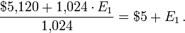
The collective average payout is therefore $5,120(Until the arrow sign) + 1,024 x E₁, and the per-game average payout is:

$\frac{$\text{5,120} + \text{1,024} \cdot E_1}{\text{1,024}} = $5 + E_1 \,.$

Because the finite contribution from n games is proportional to log₂ n, doubling the number of games played leads to a $0.50 increase in the finite contribution. For example, if 2,048 games are played, the finite contribution is $5.50 rather than $5.

It follows that, in order to be reasonably confident of achieving target average per-game winnings of approximately W (where W > $1), we should play approximately 4^W games. This will yield a finite contribution equal to W. Unfortunately, the number of games required to be confident of meeting even modest targets is astronomically high. $7 requires approximately 16,000 games, $10 requires approximately 1 million games, and $20 requires approximately 1 trillion games.

[edit] Further discussions

The St. Petersburg paradox and the theory of marginal utility have been highly disputed in the past. For a discussion from the point of view of a philosopher, see (Martin, 2004).

Power and Responsibility

Sunday, January 31, 2010

圣彼得堡悖论